TL;DR
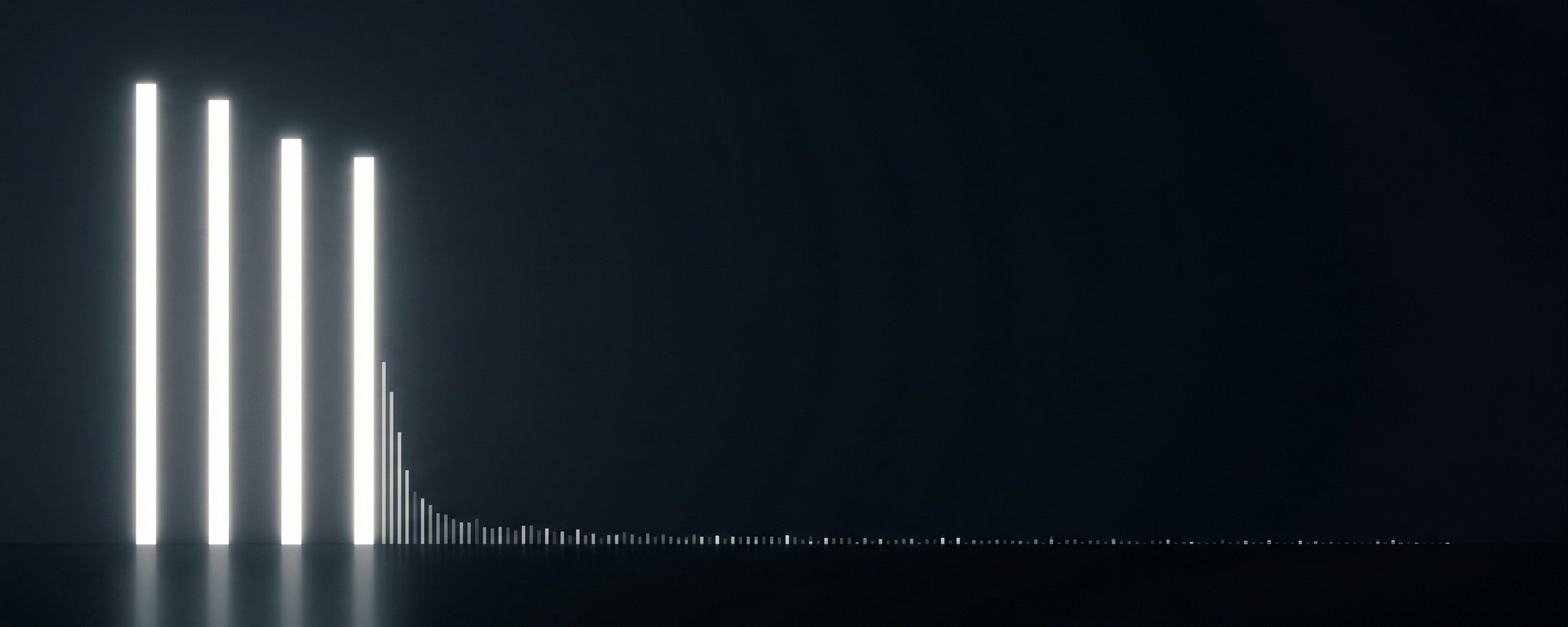
Only 4 out of 128 dimensions in the KV cache carry meaningful signal. The other 124 are noise. This holds across six models in four families.
Removing error correction on those noise dimensions improves quality, because correcting noise just injects more noise.
SpectralQuant exploits this structure: 5.95x compression (vs TurboQuant's provably near-optimal 5.02x), 4.5x faster attention, identical text quality, 15 seconds of one-time calibration.
Keys and values are fundamentally different objects: keys concentrate in ~4 dimensions, values spread across ~50. Prior work has noticed this asymmetry in various forms; we provide the precise spectral characterization and show how it dictates where error correction helps versus hurts.
We found that removing error correction from a compression algorithm makes it better. That sounds wrong, so let me explain. Think of spell-check. Running spell-check on a paragraph of real English catches real typos. Running the same spell-check on a string of random characters produces garbage: it "corrects" gibberish into wrong words with high confidence. TurboQuant, Google's KV cache compression algorithm, runs spell-check on all 128 dimensions. We discovered that 124 of those dimensions are random characters. SpectralQuant only spell-checks the 4 dimensions that contain real words. The result: 18.6% less memory on top of what Google had already “proven was near-optimal”, 4.5x faster attention decoding, and identical text quality, from 15 seconds of one-time calibration.
But to understand why this matters, you need to understand what TurboQuant did, and what it did to the market.
The TurboQuant moment
On March 24, 2026, Google Research published TurboQuant, a compression algorithm for a part of language models called the KV cache. The KV cache is essentially a notebook that the model writes in as it reads your prompt: for every word it processes, it jots down two vectors (lists of 128 numbers) per layer, so it can look back at what it already read without redoing all the work. The problem is that this notebook gets huge. At 8,000 words of context, a single 14-billion-parameter model accumulates 320 MB of notes. Scale that to a thousand users chatting at once, and memory becomes the bottleneck, not compute.
TurboQuant's approach was elegant. It compresses the notebook entries by scrambling them with a random rotation (mixing all 128 numbers together in a reversible way), then rounding each number to one of a few discrete levels (quantization), then adding an error-correction layer to fix the rounding mistakes. The whole thing requires zero setup: no looking at data, no calibration, no per-model tuning. And Zandieh, Daliri, Hadian, and Mirrokni proved that no method operating under the same "never look at the data" constraint can do substantially better. It is provably within 2.7x of the theoretical best. In other words, Google's team had not just built a good compressor; they had mathematically closed the door on doing much better. The community treated TurboQuant as the ceiling.
The paper was presented at ICLR 2026 and the reaction was immediate. Within 48 hours, multiple open-source implementations appeared. The llama.cpp community began integration work. Tom's Hardware ran coverage. But the real shockwave was financial. TurboQuant effectively proved that you could serve the same models with dramatically less GPU memory, which meant every company that had been buying expensive high-memory GPUs to handle KV cache bloat was suddenly overprovisioned. The implication rippled through GPU memory suppliers and the inference hardware stack: if software can compress the bottleneck away, the premium on memory capacity drops. Estimates of the valuation impact ranged into the tens of billions across the semiconductor supply chain. A single compression paper moved markets because it changed the economics of inference at scale.
SpectralQuant builds on TurboQuant's foundation and asks a simple question: what if 15 seconds of setup is worth it?
The answer: it is. SpectralQuant achieves 5.95x compression (vs TurboQuant's 5.02x), +2.59 percentage points better reconstruction fidelity on Qwen 2.5-14B, and 4.5x faster attention decoding. Remember: TurboQuant's 5.02x was already proven to be near the theoretical limit for any method that does not look at the data. The 18.6% compression improvement over that bound is not 18.6% over some naive baseline; it is 18.6% beyond a result that Google proved was close to optimal. The model produces identical text quality either way. The total cost of being data-aware instead of data-oblivious: 15 seconds of one-time calibration, run once before you deploy. But along the way, we discovered something we did not expect, something that tells us about how transformers actually organize information internally. More on that below.
Code is at https://github.com/Dynamis-Labs/spectralquant
The discovery: 97% of dimensions are noise
TurboQuant treats all 128 dimensions of each KV vector identically. That is what makes it data-oblivious, and that is what earns it the 2.7x optimality guarantee: a mathematical proof that no method playing by the same rules can do much better. The community took this to mean the compression problem was essentially solved. But what if those 128 dimensions are not equally important?
To find out, we looked at what the model's notebook entries actually look like. We collected thousands of key vectors from four different models, stacked them up, and asked: how many independent directions do these vectors actually point in? If all 128 dimensions carried unique information, you would need all 128 to describe the data. But if the vectors mostly cluster along a few directions and barely use the rest, then most dimensions are dead weight. We measured this using something called the participation ratio, which is essentially a count of "how many dimensions are doing real work." A participation ratio of 128 means every dimension matters equally. A participation ratio of 4 means only 4 dimensions carry meaningful information, and the other 124 are noise.
The effective dimensionality of the KV cache is d_eff ≈ 4 out of 128 dimensions, across all models, all layers, and both architectural families. Only 3.1% of dimensions carry meaningful signal. The remaining 96.9% are dominated by noise.
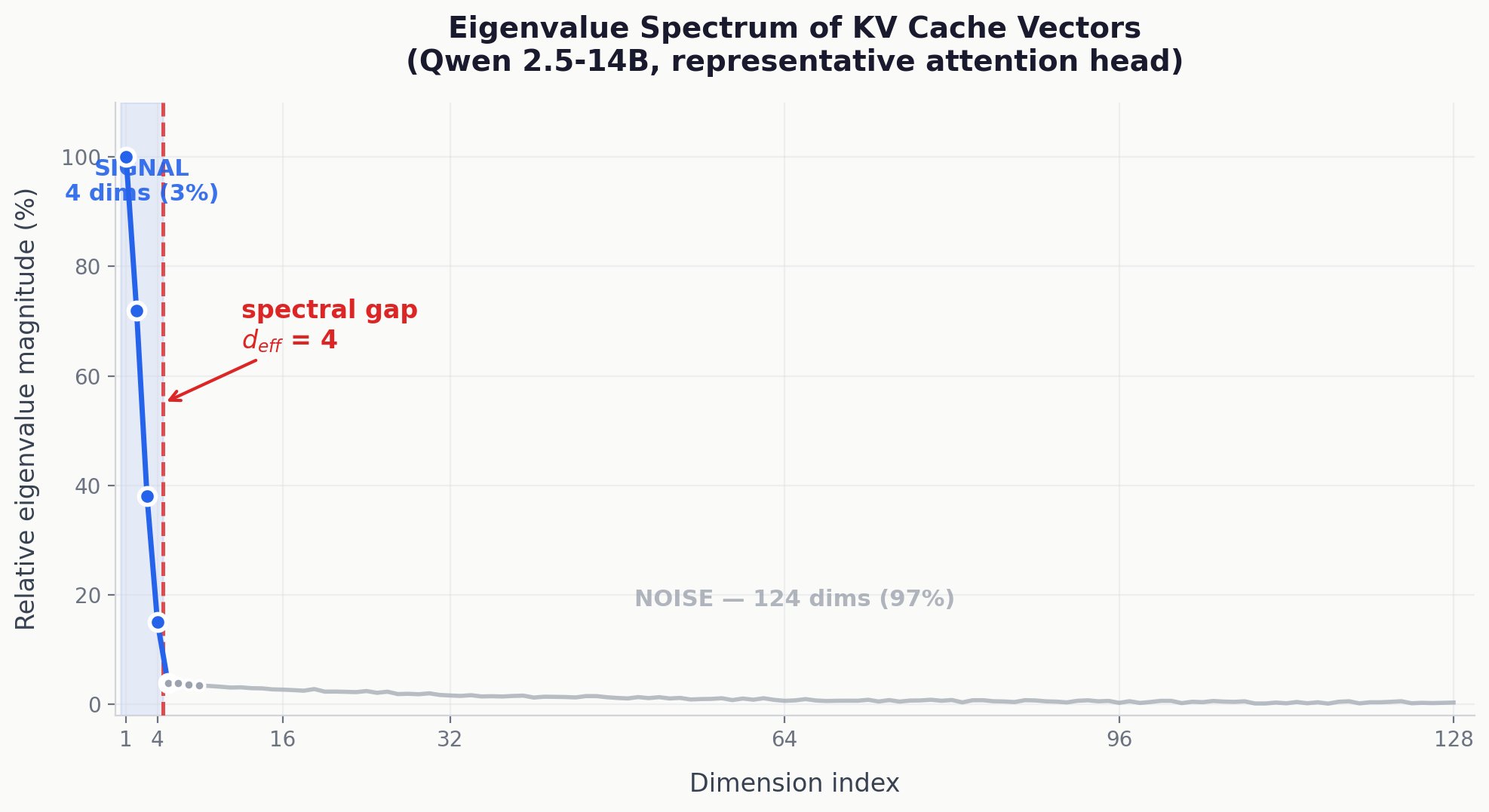
The eigenvalue spectrum of KV cache key vectors for a representative attention head in Qwen 2.5-14B. The first 4 dimensions (3%) carry nearly all the signal. The remaining 124 dimensions (97%) carry less than 3% of total variance. This cliff, the spectral gap, is what SpectralQuant exploits.
The chart above shows the eigenvalue spectrum (a ranking of how much information each dimension carries) for a representative attention head in Qwen 2.5-14B. The first four dimensions dominate. After that, there is a cliff. Dimensions 5 through 128 carry almost nothing. This cliff is what we call the spectral gap, and it means 97% of the notebook is filled with noise that TurboQuant diligently compresses and error-corrects at full precision.
This finding is remarkably consistent across models:
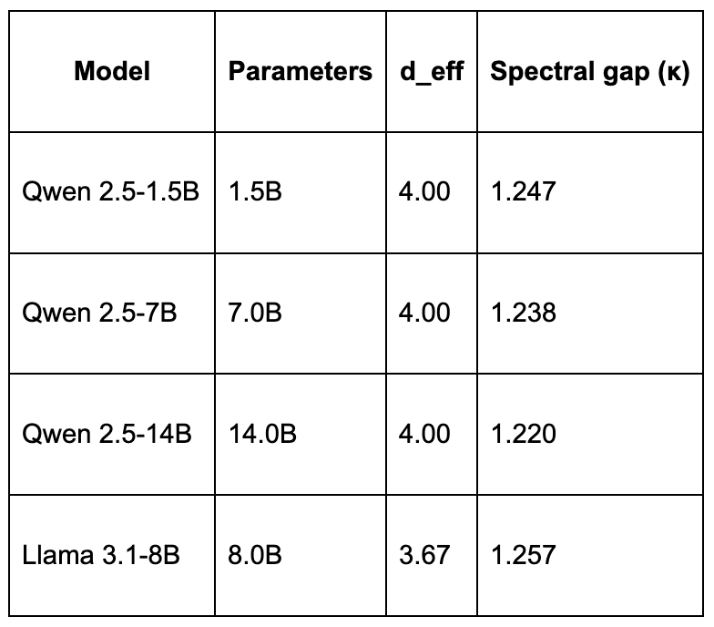
Two different model families (Qwen and Llama), a nearly 10x range of parameter counts, and the answer is the same: about 4 dimensions matter. This appears to be a structural property of how transformers organize information in their attention heads, not a quirk of any particular architecture.
How SpectralQuant works
SpectralQuant modifies TurboQuant in three targeted ways, each motivated by the spectral structure described above.
1. Spectral rotation instead of random rotation. TurboQuant scrambles the 128 dimensions using a random rotation matrix (think of it as randomly mixing all the numbers together so no single number is special). SpectralQuant instead uses a rotation learned from calibration data that lines up the coordinate system with the directions that actually carry signal. After this rotation, the first 4 coordinates contain the important stuff and the remaining 124 contain noise. The computational cost is identical: both are a 128x128 matrix multiply. The only difference is that our matrix comes from 15 seconds of looking at data, not from a random number generator.
2. Selective error correction. TurboQuant applies its error-correction step (called QJL, a technique based on random projections that estimates and fixes rounding mistakes) to all 128 dimensions, costing 128 extra bits per key vector. SpectralQuant applies error correction only to the 4 signal dimensions, saving 124 bits per key. This is where most of the memory savings come from.
3. Non-uniform bit allocation. We give more quantization precision (more rounding levels) to signal dimensions and less to noise dimensions. This follows a classical idea from information theory called water-filling: pour your bit budget where the signal is, not where it isn't.
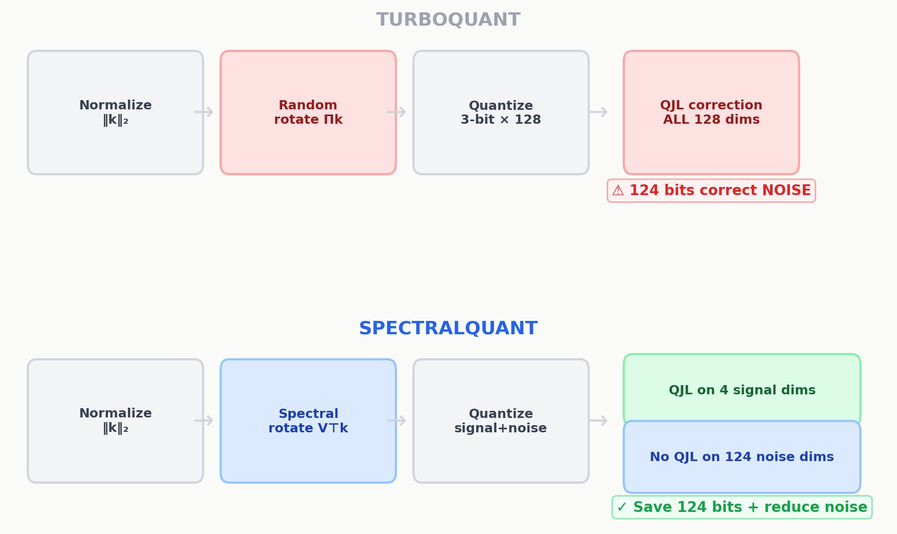
TurboQuant (top) applies error correction to all 128 dimensions, spending 124 bits correcting noise. SpectralQuant (bottom) applies error correction only to the 4 signal dimensions, saving 124 bits per key vector while actually improving reconstruction quality.
The pipeline comparison makes the difference concrete. TurboQuant (top) applies error correction to all 128 dimensions, including 124 that carry noise. SpectralQuant (bottom) applies it only to the 4 that carry signal. The rotation step costs the same either way. The only real difference is that our rotation matrix is computed from 15 seconds of calibration rather than sampled randomly.
Why does removing error correction improve quality?
This is the most counterintuitive finding in the paper, so let me walk through it carefully.
TurboQuant's error-correction step (QJL) is designed to fix the mistakes introduced by rounding. After you round each number to a discrete level, you have introduced small errors. QJL estimates those errors using a random projection (a quick, compressed snapshot of the original vector) and subtracts them out. On average, this correction is perfect: it is provably unbiased, meaning the expected correction equals the true error. But "correct on average" does not mean "helpful in every case."
On a signal dimension, rounding introduces a real error because the true value was large and meaningful. The QJL correction estimates that error and reduces it. Yes, the estimate itself is a bit noisy (it comes from a random projection, after all), but the noise is small compared to the error it fixes. Net effect: helpful.
On a noise dimension, the true value is already close to zero. Rounding a near-zero value introduces almost no error. But QJL still tries to estimate and correct that near-zero error, and the estimation process is inherently noisy. You end up adding random noise to a dimension that was already fine. Net effect: you made it worse.
Our ablation confirms this directly. Removing QJL entirely, even with a random rotation and no calibration at all, improves cosine similarity (a measure of how faithfully the compressed vectors match the originals) by +3.0 percentage points over TurboQuant. The quality gain comes primarily from removing error correction on noise, not from using a smarter rotation. The smart rotation tells us which dimensions are noise, which is what lets us save memory. But the quality improvement is from dropping the correction.
Results
We evaluated SpectralQuant across seven axes: reconstruction fidelity, perplexity (how surprised the model is by real text, a standard measure of language model quality), needle-in-a-haystack retrieval (can the model find a specific fact buried in a long document?), long-context quality, distribution shift robustness, latency, and LongBench end-task performance. The consistent finding: SpectralQuant matches or exceeds TurboQuant on every dimension.
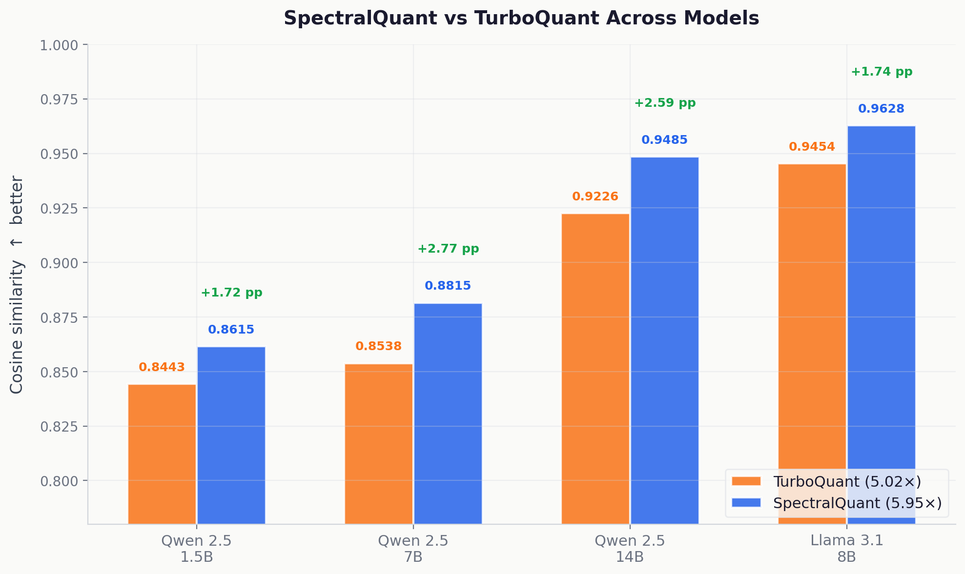
Cosine similarity across four models. SpectralQuant (blue) achieves +1.72 to +2.77 percentage points higher fidelity than TurboQuant (orange) on every model, while simultaneously compressing 18.6% further beyond TurboQuant's provably near-optimal bound.
SpectralQuant (blue) achieves higher cosine similarity than TurboQuant (orange) on all four models, with gains of +1.72 to +2.77 percentage points, while simultaneously achieving an 18.6% better compression ratio (5.95x vs 5.02x) over what Google had proven was near the theoretical limit.
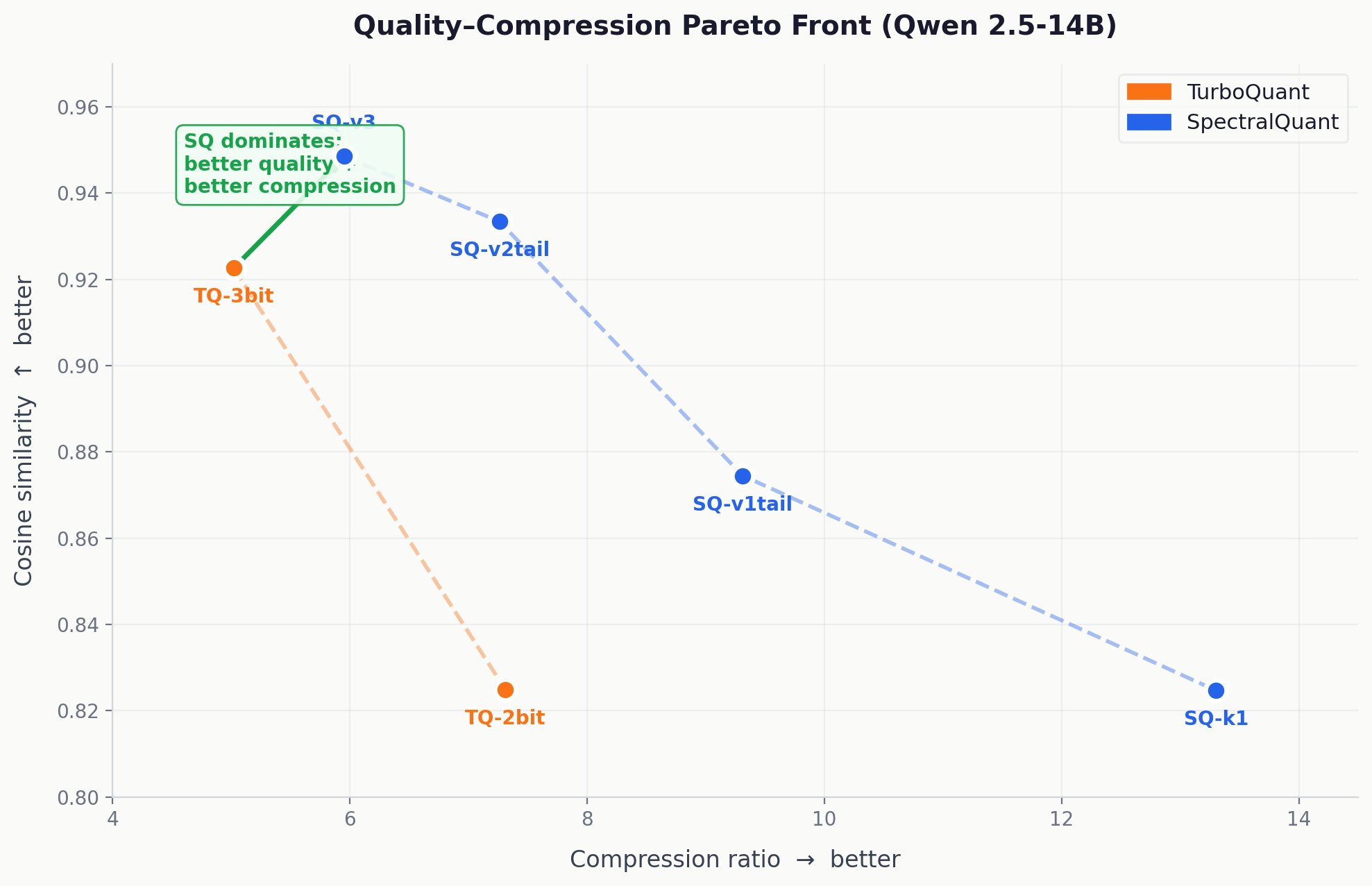
The quality-compression Pareto front on Qwen 2.5-14B. Each point is one compression configuration. SpectralQuant configurations (blue) dominate TurboQuant configurations (orange): higher quality and better compression simultaneously. SQ-v3 achieves strictly better quality AND better compression than TQ-3bit. There is no tradeoff.
The Pareto front (a plot that shows the best achievable quality at each compression level) tells the full story. Each point is one compression configuration on Qwen 2.5-14B. SpectralQuant configurations (blue) consistently dominate TurboQuant configurations (orange). They are higher (better quality) and further right (better compression). The SQ-v3 point achieves strictly better quality AND better compression than TQ-3bit. There is no tradeoff here.
Does compression affect generation quality?
Cosine similarity measures how faithfully we reconstruct each vector. But does that actually change the text the model generates? We measured three things that matter for deployment:
Perplexity: 9.51 for all methods. FP16 (full precision, no compression), TurboQuant, and SpectralQuant all produce identical perplexity. The model generates the same quality text regardless of compression method. This means SpectralQuant's cosine similarity improvement does not translate to measurably better text. Rather, it means we are achieving compression neutrality (same text quality) at less memory and faster speed.
Needle-in-a-haystack: 10/10 for all methods. We inserted a specific fact (a random phone number) at various positions in a long document and asked the model to retrieve it. Both TurboQuant and SpectralQuant achieve perfect retrieval at context lengths up to 8,192 tokens. Compression does not cause the model to "forget" anything.
Attention speedup: 4.5x. Because SpectralQuant skips the QJL computation at decode time (there is nothing to correct on 124 dimensions), attention runs 4.5x faster than TurboQuant.
SpectralQuant's practical value proposition is: identical generation quality at 18.6% less memory than what was already proven near-optimal, and 4.5x faster attention decoding. For inference teams, this is the right result. You want compression that does not degrade your model. SpectralQuant does not, while using fewer resources.
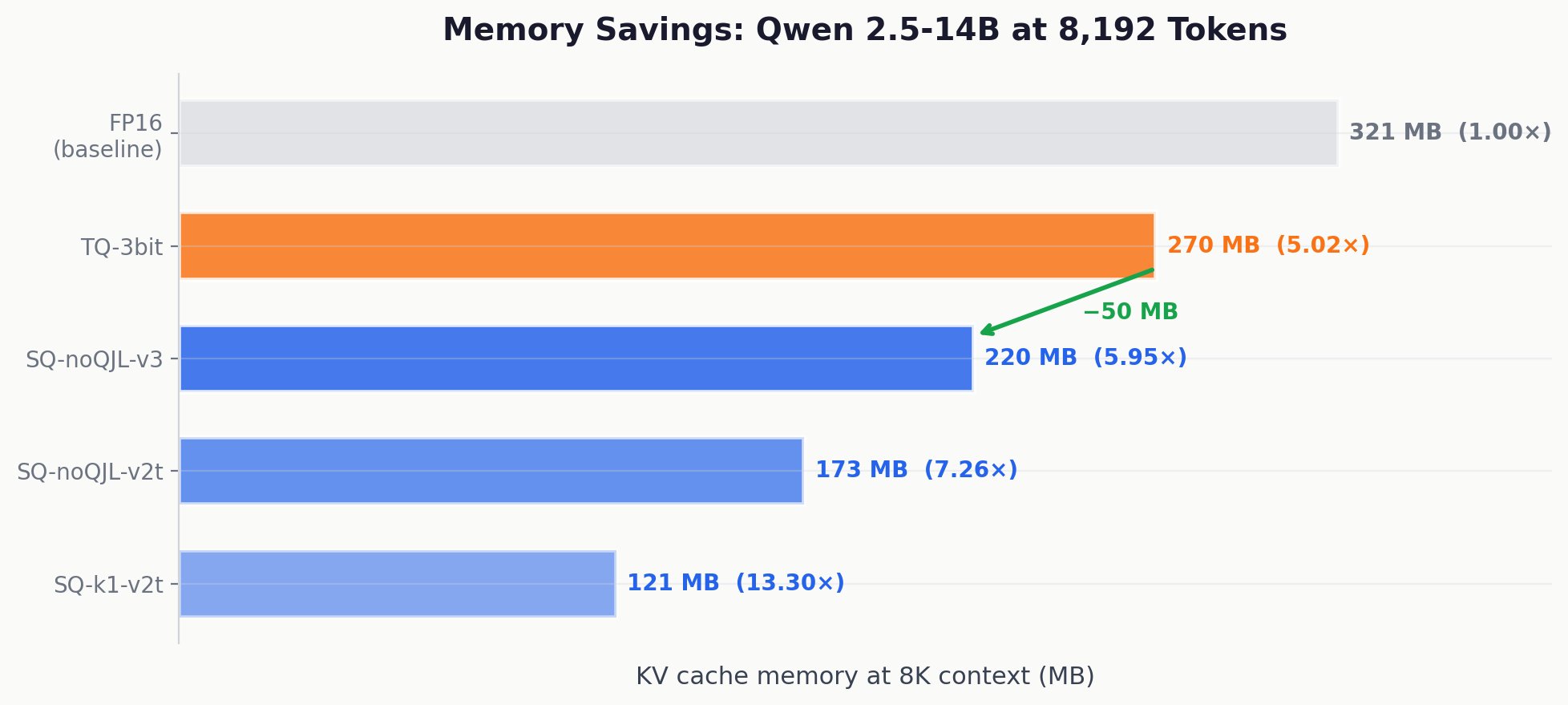
KV cache memory at 8,192 tokens on Qwen 2.5-14B. SpectralQuant (SQ-noQJL-v3) saves 50 MB over TurboQuant's already compressed baseline, with more aggressive configurations saving up to 200 MB. All SpectralQuant configurations maintain equal or better reconstruction quality.
Statistical reliability
We repeated the comparison across five independent random seeds (different random data shuffles and initialization). SpectralQuant won all five, with mean cosine similarity 0.8681 ± 0.0013 versus TurboQuant's 0.8404 ± 0.0043. SpectralQuant is not only higher on average but 3.3x more consistent across runs.
Distribution shift
SpectralQuant calibrates on WikiText-2, a dataset of encyclopedia text. But what if you deploy the model on code, or chat, or legal documents? We tested cross-domain evaluation: calibrating on code and evaluating on natural language, and vice versa. SpectralQuant's advantage held across all four domain combinations, with gains from +2.1 to +3.6 percentage points. The calibration captures structural properties of the model itself, not surface features of any particular text domain. You calibrate once and it works on everything.
The experiment that failed, and why it matters more than the one that worked
Here is where the story takes a turn. We found that only 4 out of 128 dimensions carry signal in the keys. The natural next question is obvious: why bother storing the other 124 at all? Instead of compressing all 128 dimensions with quantization, just keep the 4 that matter. Project each key onto those 4 directions, store 4 numbers instead of 128. That would give you 25.6x compression, five times better than TurboQuant, with no quantization noise at all. No codebooks, no bit packing, no rounding errors. Just 4 clean numbers.
We tried it. It did not work. And the reason it did not work reveals something fundamental about how transformers process information.
Keys concentrate, values do not
The KV cache stores two things per token: a key (which determines how much attention a token receives) and a value (which determines what information gets passed forward when a token is attended to). We had been measuring the spectral structure of keys. When we measured values separately, we found something completely different.
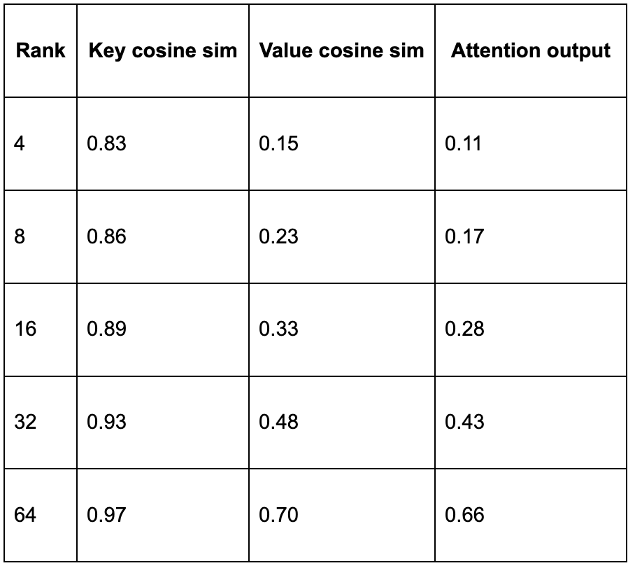
At rank 4, keys reconstruct reasonably well (0.83 cosine similarity). Values are catastrophic (0.15). Even at rank 64, which only gives you 2x compression, the attention output quality (0.66) is still far below TurboQuant's 0.84 at 5x compression. Keys live in 4 dimensions. Values live in many more. The spectral concentration we found is a property of keys specifically, not of the KV cache in general.
Why the asymmetry?
Think about what keys and values actually do in the attention mechanism.
Keys answer the question: "How relevant is this token to what we are looking for right now?" This is fundamentally a matching problem. The model computes a dot product between the current query and every cached key to decide which tokens to pay attention to. For this matching to work, keys need to live in the same low-dimensional subspace that queries live in. If the model learns that "relevance" can be captured along 4 principal directions (say: topic, syntax, position, and some learned feature), then all keys will align to those directions. The population of keys concentrates, giving you d_eff = 4.
Values answer a different question: "Given that this token is relevant, what information should it contribute?" This is fundamentally a diversity problem. Each token needs to contribute different information to the output. A noun contributes different value content than a verb. A number contributes differently than a preposition. If all values clustered in 4 dimensions, the model could only express 4 types of information in its output, which would be crippling. So values spread out across many dimensions, each token pointing in its own direction.
Here is the subtle part. The participation ratio measures how the population variance is distributed across dimensions. For keys, most of the population's variance is in 4 directions because all keys cluster there. For values, the variance is spread out because different tokens use different dimensions. But this does not mean individual value vectors are high-dimensional. Each individual value vector might be relatively simple. The point is that different value vectors are simple in different directions. The population looks high-dimensional because the diversity across tokens uses the full space, even though each individual token only uses a small part of it.
This is the difference between concentration and diversity. Keys concentrate (same few directions, high variance there, low everywhere else). Values diversify (each vector uses its own directions, so the average variance is spread thin across all of them). Truncation kills diversity. Quantization preserves it, because quantization keeps all dimensions, just at lower precision.
What this tells us about transformers
This asymmetry has been observed before in various forms. KIVI (ICML 2024) showed that keys and values need different quantization strategies based on different outlier patterns. Loki (2024) exploited low-rank structure in keys specifically. The "Homogeneous Keys, Heterogeneous Values" paper (Cui and Xu, 2025) documented the asymmetry in attention weight distributions, and KV-CoRE (2026) measured that keys have substantially lower effective rank than values. What we add is a precise spectral characterization: d_eff ≈ 4 for keys versus approximately 50 for values, stable at a 3% ratio across model families and scales, and the connection between this structure and where error correction helps versus where it hurts. The asymmetry says something specific about how transformer attention layers organize their internal representations.
Attention heads are narrow selectors but broad readers. The selection mechanism (keys and queries) operates in a low-dimensional subspace, because the notion of "relevance" for any given head is simple and consistent across tokens. But the information retrieval mechanism (values) operates in a much higher-dimensional space, because the content that different tokens contribute is diverse and cannot be compressed into a few directions. This has implications beyond compression. It suggests that key projection matrices are implicitly low-rank: the weight matrix that produces keys (W_K) effectively projects the high-dimensional residual stream (5,120 dimensions in a 14B model) down to just 4 effective dimensions, even though the nominal key dimension is 128. The other 124 dimensions of the key are noise from the perspective of what the key projection learned to represent. Value projection matrices, by contrast, are full-rank or close to it, because they need to represent diverse information across different tokens. And perhaps most intriguingly, the number 4 might tell us something about the complexity of "relevance" itself: if d_eff = 4 universally across model sizes and families, it might reflect the intrinsic complexity of the relevance matching problem in natural language. How many independent axes of "relevance" does an attention head need? Apparently about four. We plan to investigate this further in follow-up work.
The practical lesson
The low-rank experiment taught us what the spectral structure is and what it is not. It is a guide for bit allocation: the d_eff = 4 finding tells you where to put your bits (on the signal dimensions) and where to skip error correction (on the noise dimensions). That is exactly what SpectralQuant does, and it works. It is not a license to throw away dimensions. Variance concentration across the population does not mean individual vectors are low-dimensional. Values prove this directly: each value vector needs its own set of dimensions, and truncating to the population's principal components destroys per-token information that the model relies on.
SpectralQuant quantizes all 128 dimensions rather than truncating to d_eff, because quantization preserves all dimensions at lower precision while truncation obliterates 124 of them entirely. The spectral structure tells you how to quantize intelligently, not what to discard.
What does this mean?
TurboQuant proved something important: you can get surprisingly good compression without ever looking at your data. That is a real theoretical achievement, and the 2.7x optimality bound is tight. No data-oblivious method will substantially beat it. The community reasonably treated this as a closed problem. SpectralQuant shows that the problem was only closed if you accept the constraint of never looking at your data. Nearly all of the distance between "data-oblivious optimal" and "actually optimal" concentrates in one place: the difference between treating every dimension equally and recognizing that 97% of them carry noise. Closing that gap costs 15 seconds of one-time calibration. In exchange, you get 18.6% less memory beyond the proven near-optimal bound, 4.5x faster attention, and identical text quality.
The insight generalizes beyond KV caches. Any compression pipeline that applies uniform error correction to data where most dimensions carry noise will face the same problem: correction on low-signal dimensions injects noise without fixing anything. The fix is always the same. Measure the spectral structure (cheaply), then allocate corrections proportionally to where the signal actually is.
And then there is the structural finding that ties everything together. Keys and values are fundamentally different objects, even though they are stored side by side in the same cache. Keys are narrow: they select along a few consistent directions. Values are broad: they carry diverse information that cannot be reduced. Others have noticed this asymmetry before, and several compression methods already treat keys and values differently. Our contribution is making it precise and exploitable: the participation ratio gives you a single number (d_eff ≈ 4 for keys, approximately 50 for values) that tells you exactly where to allocate bits and where to skip error correction. Any future compression method that treats keys and values with the same error-correction budget is leaving something on the table.
The number 4 (d_eff ≈ 4, universal across model families and scales) probably tells us something about the intrinsic complexity of attention-based relevance matching in natural language. We do not fully understand why yet. But the fact that it is stable, measurable, and exploitable suggests it is worth understanding.
Try it
SpectralQuant is open source. Calibration takes 15 seconds on a single GPU.
git clone https://github.com/Dynamis-Labs/spectralquant
cd spectralquant && pip install -e ".[dev]"
python scripts/calibrate.py --model Qwen/Qwen2.5-14B-Instruct
# ≈ 15 seconds → eigenvectors saved
python experiments/eval_memory_efficiency.py --config SQ_noQJL_v3
# Expected: cos_sim = 0.9485, ratio = 5.95×
Repo: https://github.com/Dynamis-Labs/spectralquant
Paper: https://github.com/Dynamis-Labs/spectralquant/blob/main/paper_output/spectralquant.pdf [Will update with Arxiv link when its available]
About Sentra
Sentra is building enterprise general intelligence: a shared AI layer that sits on all communication channels and agent traces to understand how everyone in an organization actually works and how work actually gets done. From these interactions, Sentra builds a living world model of the entire company in near real time. The central insight is that every piece of knowledge created in an organization originates from interactions between humans, agents, or both. By tapping into that primary layer rather than forcing teams to maintain separate systems of record, Sentra constructs an all-knowing representation of the organization itself, a collective consciousness that anyone can query, from the CEO wanting full visibility across the company to an individual contributor needing context for a decision.
SpectralQuant (this work) grew directly out of this work. While building Sentra's world model, we discovered that learned representations occupy far fewer effective dimensions than their nominal size, and we were exploiting that spectral structure to store organizational knowledge more efficiently. That observation is what led us to ask the same question about the KV cache, and the answer turned out to be the same: 97% of the space is noise.
Sentra is funded by a16z Speedrun and Together Fund.
SpectralQuant builds directly on TurboQuant by Zandieh, Daliri, Hadian, and Mirrokni (ICLR 2026) and our own work “Price of meaning” by Sambarta, Andrey, Sofia, Nikhil, and Ashwin (Arxiv). We thank Anirudh Bharadwaj Vangara for the community TurboQuant implementation used as our baseline. Experiments were conducted on NVIDIA B200 hardware via Modal.